PaddockTS

Paddock-scale time-series analysis of Australian agricultural land, end-to-end from a single bounding box.

PaddockTS takes a time and region of interest and produces paddock (or field) boundaries, paddock-level time series of vegetation indices and fractional ground cover, seasonal phenology metrics, and matched terrain, climate, and soil data, together with plots, videos, and a PDF report.

Built at the Borevitz Lab, Australian National University for ecologists, agronomists, and remote-sensing researchers who want a reproducible pipeline from Sentinel-2 imagery to paddock boundaries and paddock-level summaries of greenness, ground cover, and phenology.

---

What you get

Given a Troi (Time and Region Of Interest — a bounding box and a date range), get_outputs(troi) produces the outputs described below. The examples on this page are from an eight-year run (2018–2025) over the Milgadara farm, New South Wales:

True-colour Sentinel-2 observations, 2018–2025, with automatically segmented paddock boundaries

Fractional cover for the same period: red = bare ground, green = green vegetation, blue = non-green vegetation

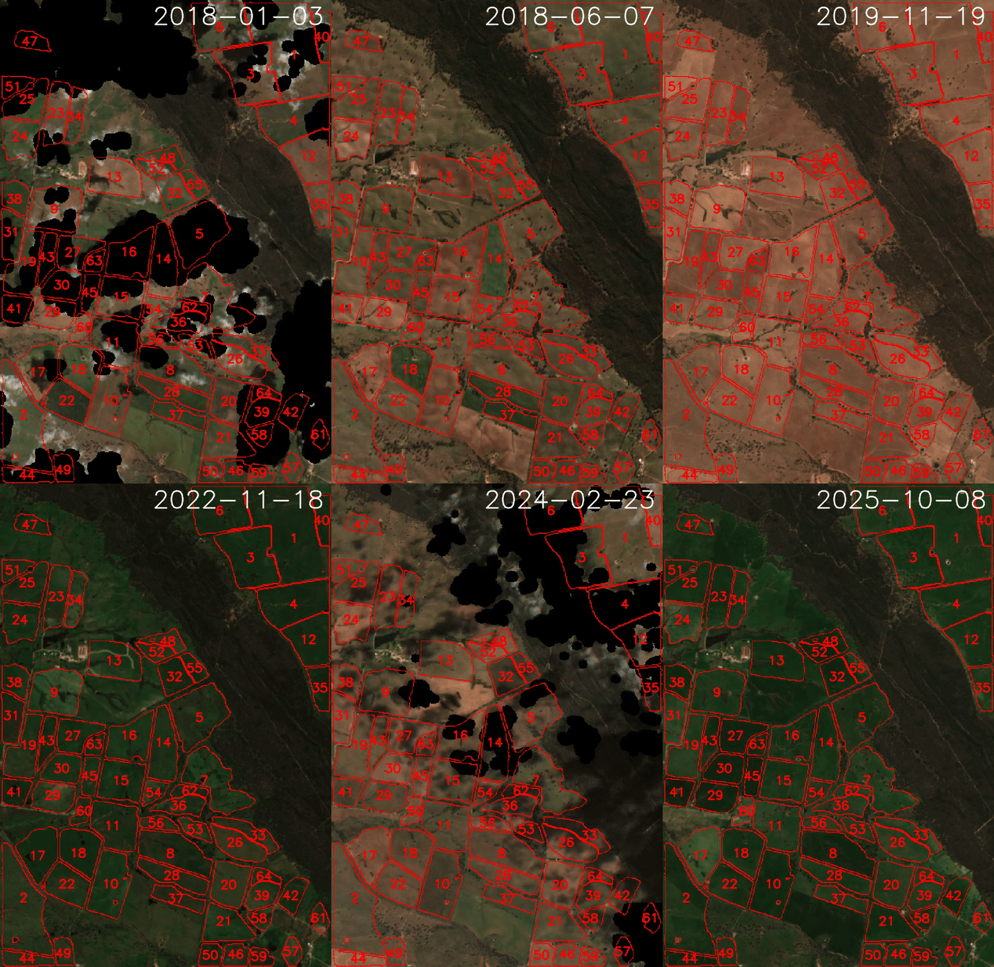
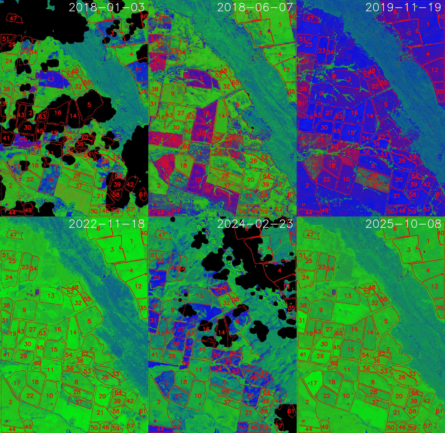
Paddock boundaries

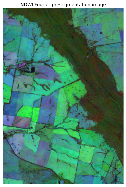
Field boundaries are segmented automatically. The Sentinel-2 stack is condensed into a single NDWI Fourier-feature image, in which persistent field boundaries are emphasised and transient patterns suppressed; Segment Anything segments this image, and the resulting masks are exploded, reprojected, and filtered by area and isoperimetric compactness. The output is a GeoPackage with paddock geometries, identifiers, area_ha, and compactness. User-supplied boundaries can be analysed instead of, or alongside, the segmented ones — see Bring your own paddocks.

NDWI Fourier-feature presegmentation image

Filtered segmentation result over true-colour imagery

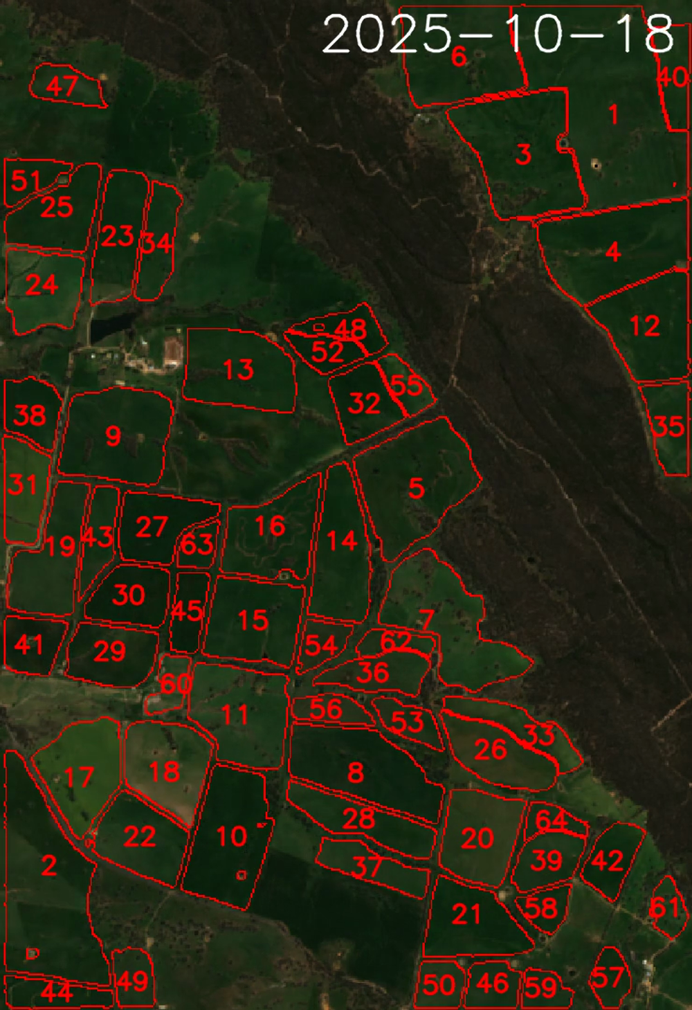
Per-paddock time series

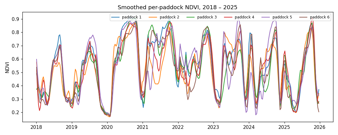
For each clear acquisition, the NaN-aware median of every Sentinel-2 band, the five spectral indices (NDVI, CFI, NIRv, NDTI, CAI), and the fractional-cover fractions is computed within each polygon and stored as a Zarr dataset on (paddock, time). A resampled, gap-filled, Savitzky–Golay-smoothed variant is used for phenology and plotting.

Smoothed per-paddock NDVI for six paddocks, 2018–2025

Fractional ground cover

Sentinel-2 reflectance is unmixed per pixel into bare ground (bg), green vegetation (pv), and non-green vegetation (npv) fractions, using a TFLite model adapted from fractionalcover3. These fractions underlie the false-colour timelines above and are included in the per-paddock time series.

Seasonal phenology

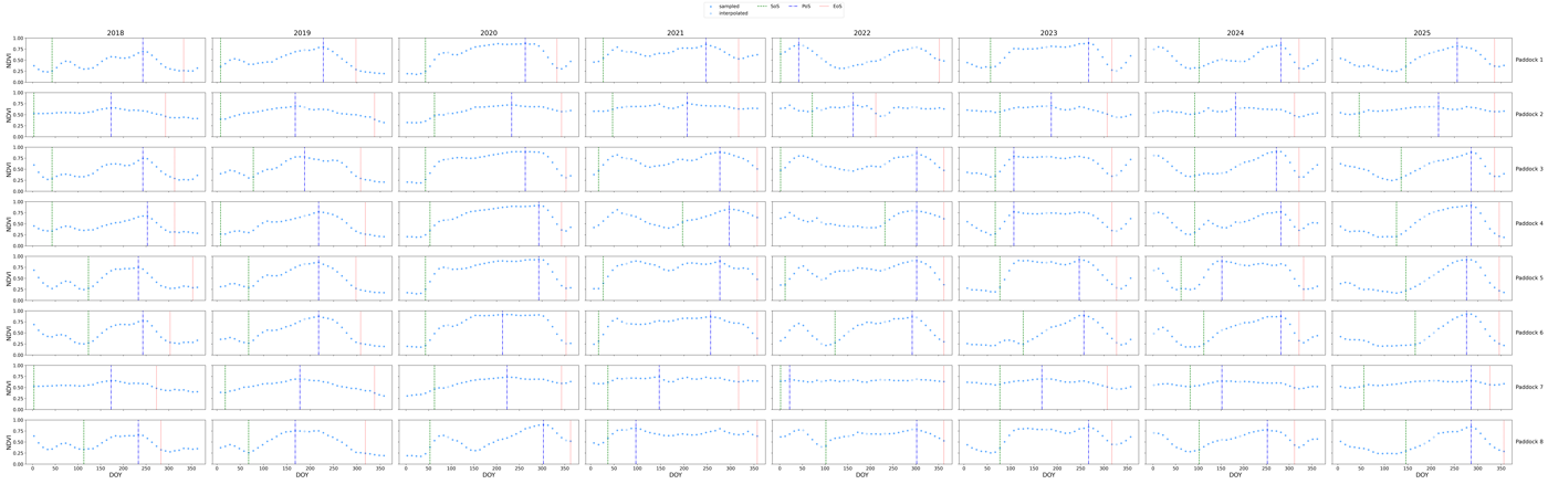
Start, peak, and end of season (day-of-year and value), seasonal amplitudes, length of season, integrals under the curve, and a peak count are computed for each paddock and year with a vendored version of phenolopy. Results are returned as DataFrames and written to a CSV covering all years.

Detected season markers on the smoothed curves, one panel per year

Paddock calendar

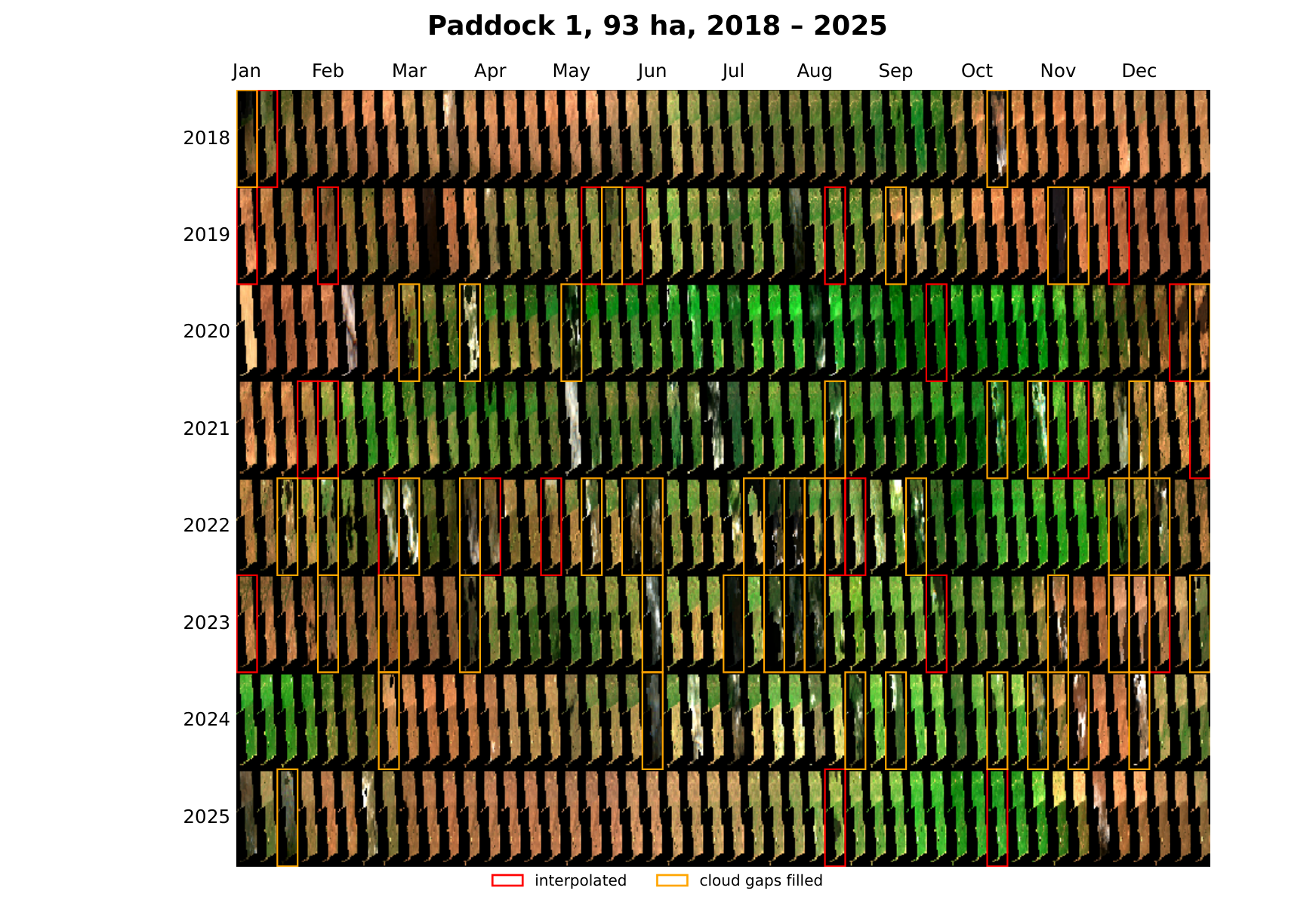
Calendar plots show one page per paddock, one row per year, and 48 thumbnail slots across the season. Slots without a clear observation are interpolated and outlined in red; mostly-clear slots whose cloud-masked pixels were gap-filled are outlined in orange.

Calendar page for one paddock over eight years; red = interpolated, orange = cloud gaps filled

Environmental context

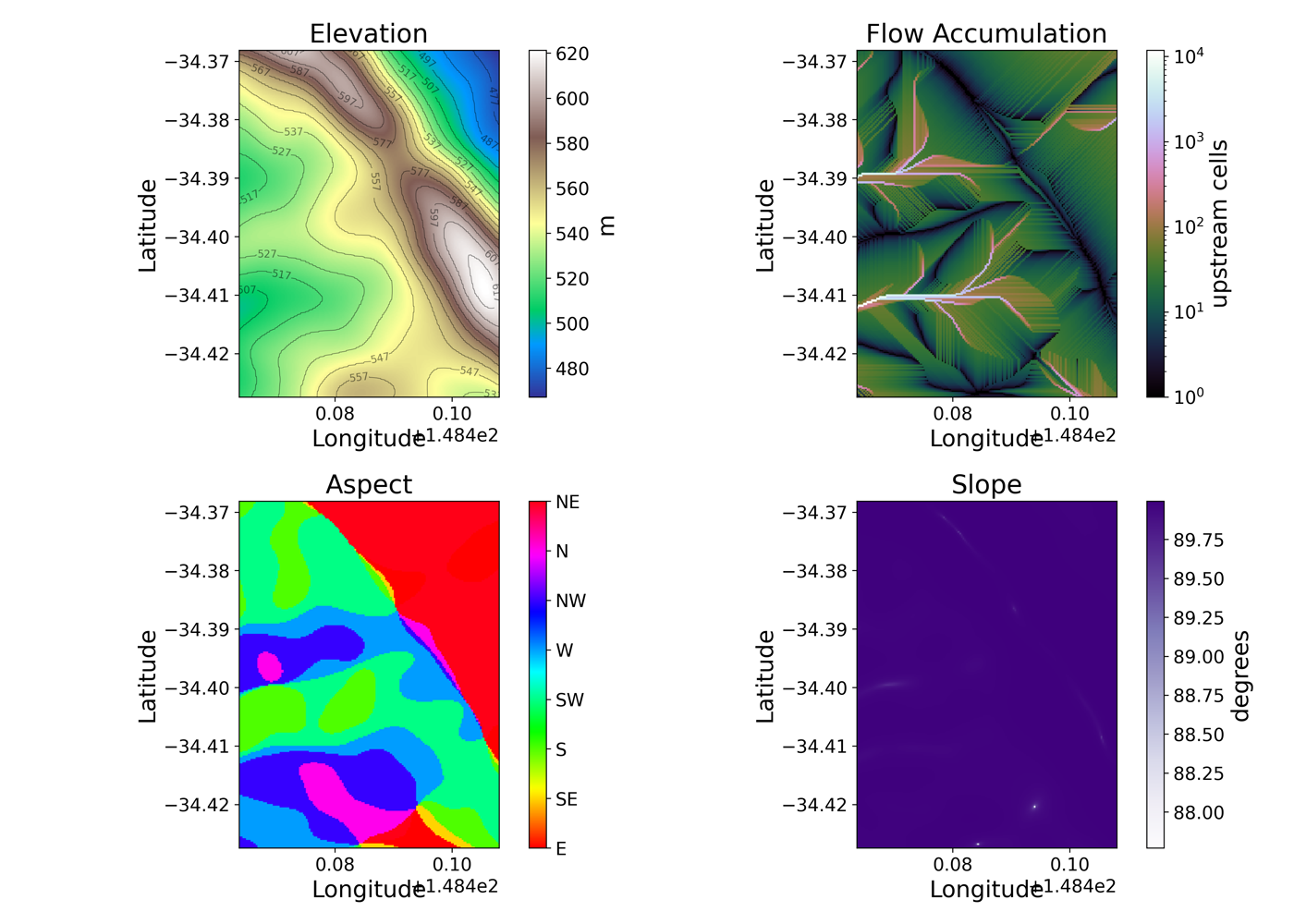
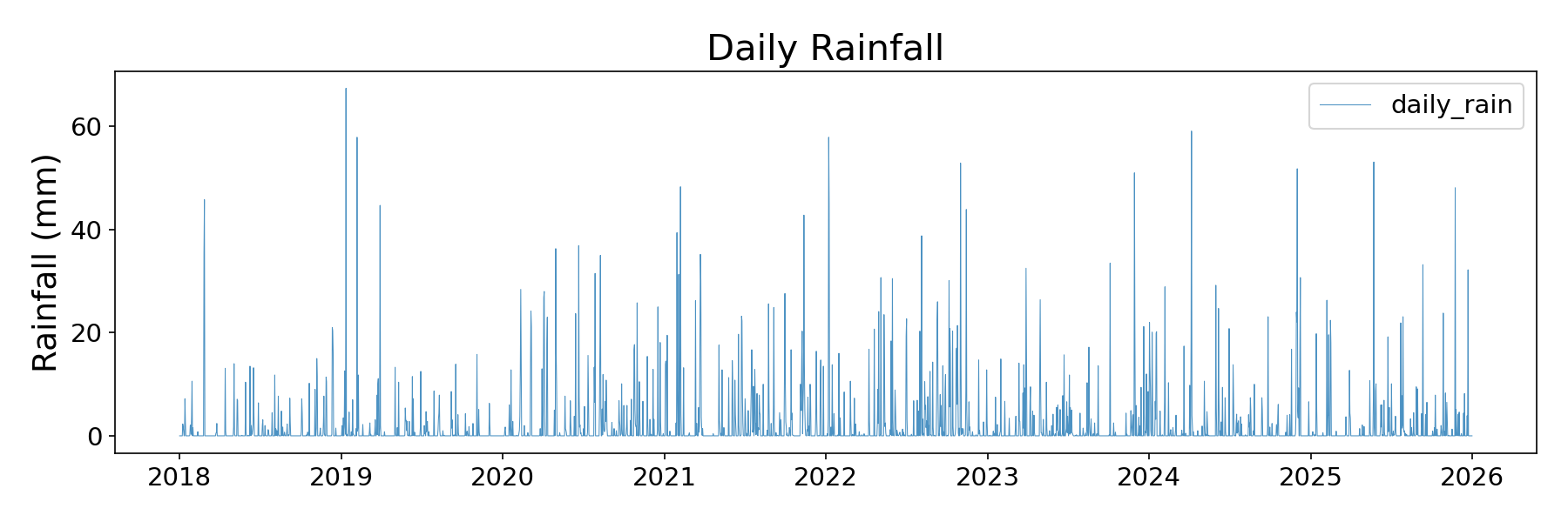
Copernicus 30 m elevation with derived slope, aspect, flow accumulation, and TWI; OzWALD and SILO daily climate; and SLGA 90 m soil properties, matched to the same area of interest. These are read through machine-wide stores that reuse previously downloaded observations across overlapping regions and dates.

DEM-derived terrain variables on the Sentinel-2 grid

SILO daily climate panels

PDF report

The topography, climate, calendar, and phenology outputs are combined into a single landscape-A4 PDF per run.

---

Quick example

from datetime import date
from troi.troi import Troi
from PaddockTS.get_outputs import get_outputs

troi = Troi(
    bbox=[148.36265, -33.52606, 148.38265, -33.50606],
    start=date(2020, 1, 1),
    end=date(2021, 12, 31),
    stub="my_first_run",
)

get_outputs(troi)

This kicks off both pipelines (Sentinel-2 → PaddockTS and Environmental) in parallel and renders a live two-column status dashboard. Outputs land under ~/Documents/Troi-Outputs/<stub>/ (configurable). The next get_outputs(troi) for the same Troi is a no-op — every stage finds its cached output and skips.

---

Bring your own paddocks

If you already have paddock boundaries from QGIS, a cadastral layer, or a previous run, skip SAM segmentation and use them directly:

from datetime import date
from troi.troi import Troi
from PaddockTS.get_outputs import get_outputs

paddocks_fp = "/path/to/my_paddocks.gpkg"  # or .geojson / .shp

troi = Troi.build_from_paddocks(
    paddocks_filepath=paddocks_fp,
    start=date(2024, 1, 1),
    end=date(2024, 12, 31),
    stub="my_farm",
    label_col="paddock_name",  # column holding human-readable names
)

get_outputs(
    troi,
    paddocks_filepath=paddocks_fp,
    skip_sam=True,
    label_col="paddock_name",
)

---

Where to go next

• Getting started — install, configure, construct a Troi, and run your first pipeline.
• Pipeline — every stage, what it produces, what it reads, what it caches, and how to skip or replace any of it.
• API reference — full signatures and runnable examples for every public function.
• Demo notebooks — three runnable Jupyter notebooks: the quickstart, calling stages individually, and using your own paddock boundaries.

---

License

PaddockTS is MIT-licensed — see LICENSE.

It vendors third-party code under permissive licenses (see PaddockTS/LICENSES/):

• fractionalcover3 — Robert Denham, MIT
• phenolopy — Lewis Trotter, Apache 2.0
• DAESIM_preprocess — Christopher Bradley, MIT

If you publish work using PaddockTS, please cite the upstream data sources (DEA Sentinel-2 ARD, Copernicus DEM, OzWALD, SILO, SLGA) and the third-party libraries above.