Pipeline
PaddockTS runs two pipelines in parallel from a single Troi:
- Sentinel-2 → PaddockTS — up to 21 stages producing paddock segmentation, time series, phenology, plots, and a stitched PDF report.
- Environmental — 7 stages pulling terrain, climate, and soil data.
PaddockTS.get_outputs.get_outputs(troi) orchestrates both on two
threads with a live rich dashboard.
flowchart TD
    Q["<b>Troi</b><br/>bbox · dates · stub"] --> GO(["get_outputs(troi)"])

    GO -->|"thread 1 · Sentinel-2 → PaddockTS"| D["Download + clean<br/>Sentinel-2"]
    D --> IDX["Spectral indices<br/>NDVI · CFI · NIRv · NDTI · CAI"]
    D --> FC["Fractional cover<br/>bg · pv · npv"]
    D --> SAM["Segment paddocks<br/>(SAM)"]
    IDX --> TS["Per-paddock<br/>time series"]
    SAM --> TS
    TS --> YR["Yearly split<br/>+ DOY"]
    YR --> PH["Phenology<br/>SoS · PoS · EoS"]
    FC --> PLOT["Videos · calendar ·<br/>phenology plots"]
    SAM --> PLOT
    PH --> PLOT

    GO -->|"thread 2 · Environmental"| TER["Terrain DEM<br/>slope · aspect · TWI"]
    GO --> OZ["OzWALD<br/>daily climate"]
    GO --> SILO["SILO<br/>climate"]
    GO --> SLGA["SLGA<br/>soils"]
    TER --> EPLOT["Climate +<br/>terrain plots"]
    OZ --> EPLOT
    SILO --> EPLOT
    SLGA --> EPLOT

    D -.->|"clean cube<br/>(terrain plot waits)"| EPLOT
    PLOT --> PDF[["Stitched PDF report"]]
    EPLOT --> PDF

    classDef default color:#000;
How a stage works
Each stage is a plain Python function that:
- takes the
Troiplus optionally a previous stage's in-memory output as a kwarg, - if that kwarg is missing, loads the previous output from disk (and cascades — generating it first if needed),
- writes its own output to a deterministic path derived from
Troi, - touches a
_SUCCESSmarker after the data write completes; the marker is the cache-validity check on the next call.
This means you can call any stage in isolation, in any order, and the
caching falls into place. get_outputs exists purely to orchestrate
the full run with progress output — none of the stage functions
require it.
get_outputs also gates downstream Sentinel-2 stages on their
upstream dependencies: if SAM segmentation (stage 5) fails, the
SAM-dependent video / TS / phenology / plot stages downstream are
marked skipped rather than running, failing on missing inputs, and
filling the dashboard with cascading errors. See
get_outputs — Cascading-skip.
Sentinel-2 → PaddockTS pipeline
The driver runs each numbered stage in order. Stages marked (SAM)
operate on the auto-segmented SAM paddocks; stages marked (user)
operate on a user-provided paddocks file passed via the
paddocks_filepath argument to get_outputs. Stages are skipped if
their inputs aren't available (e.g. skip_sam=True skips the SAM
stages, or no paddocks_filepath skips the user stages).
| # | Stage | Module | Output |
|---|---|---|---|
| 1 | Sentinel-2 window (clean) | pysentinel2.cube.Cube |
in-memory (cube-backed) |
| 2 | Spectral indices | pysentinel2.derive (on read) |
in-memory |
| 3 | Compute fractional cover | FractionalCover.compute_fractional_cover |
fractional_cover.zarr |
| 4 | Sentinel-2 video | Plotting.sentinel2_video |
{stub}_sentinel2.mp4 |
| 5 | Segment paddocks (SAM) | PaddockSegmentation.get_paddocks |
sam_paddocks.gpkg |
| 6 | S2 + paddocks video (SAM) | Plotting.sentinel2_paddocks_video |
..._sentinel2_paddocks.mp4 |
| 7 | S2 + paddocks video (user) | Plotting.sentinel2_paddocks_video |
..._sentinel2_paddocks.mp4 |
| 8 | Fractional cover video | Plotting.fractional_cover_video |
{stub}_fractional_cover.mp4 |
| 9 | FC + paddocks video (SAM) | Plotting.fractional_cover_paddocks_video |
..._fractional_cover_paddocks.mp4 |
| 10 | FC + paddocks video (user) | Plotting.fractional_cover_paddocks_video |
..._fractional_cover_paddocks.mp4 |
| 11 | Make paddock TS (SAM) | Phenology.make_paddock_time_series |
..._timeseries.zarr |
| 12 | Make paddock TS (user) | Phenology.make_paddock_time_series |
..._timeseries.zarr |
| 13 | Make yearly paddock TS (SAM) | Phenology.make_yearly_paddock_time_series |
..._timeseries_<year>.zarr |
| 14 | Make yearly paddock TS (user) | Phenology.make_yearly_paddock_time_series |
..._timeseries_<year>.zarr |
| 15 | Estimate phenology (SAM) | Phenology.estimate_phenology |
{year: DataFrame} in-memory |
| 16 | Estimate phenology (user) | Phenology.estimate_phenology |
{year: DataFrame} in-memory |
| 17 | Calendar plot (SAM) | Plotting.calendar_plot |
..._calendar_<year>_p01.png (PNG) + vector pages in the PDF report |
| 18 | Calendar plot (user) | Plotting.calendar_plot |
..._calendar_<year>_p01.png (PNG) + vector pages in the PDF report |
| 19 | Phenology plot (SAM) | Plotting.phenology_plot |
..._phenology_p01.png |
| 20 | Phenology plot (user) | Plotting.phenology_plot |
..._phenology_p01.png |
| 21 | PDF report | Plotting.make_pdf |
{stub}.pdf |
Stage 1: Sentinel-2 window (via the pysentinel2 cube)
Sentinel-2 comes from the machine-wide
pysentinel2 cube:
Cube.get_ds_troi(troi, clean=True) downloads only the pixels no
previous read has fetched (coverage is tracked per day as exact pixel
rectangles), then applies cloud masking on read. Cleaning dilates the fmask cloud/shadow (and snow) mask by
buffer_px to catch cloud-edge halos, and gates frames on
max_cloud_fraction (contamination over valid pixels) and
min_valid_fraction (swath coverage) — per-frame cloud_fraction /
valid_fraction land as coordinates on the returned dataset. See the
pysentinel2 README's Cleaning & masking section for the full design.
Failure modes specific to DEA's STAC are documented in pysentinel2's
diagnostics.md.
Stage 5: Paddock segmentation (SAM)
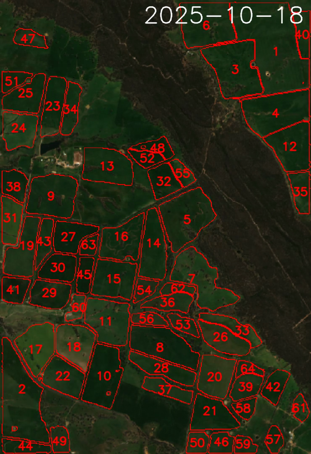 Automatically segmented paddocks over the true-colour Sentinel-2 window.
Three internal steps:
- Presegmentation (
_presegment) — derives a single grayscale image from the multi-temporal Sentinel-2 stack using NDWI Fourier features. This collapses time into a representation that emphasises stable field boundaries and suppresses transient noise (clouds, shadows, seasonal greenness). Written as a GeoTIFF atPaths(troi).preseg. - SAM mask generation — feeds the presegmented image to
segment-geospatial(default backbone: SAM ViT-H, ~2.4 GB checkpoint auto-downloaded to{config.tmp_dir}/sam_weightson first run) and writes a mask GeoTIFF plus raw polygons GeoPackage. - Vectorisation and filtering — explodes multipart geometries,
reprojects to a local UTM zone for accurate area / perimeter,
computes
area_haand isoperimetriccompactness = 4πA/L², drops polygons outside[min_area_ha, max_area_ha]or belowmin_compactness, sorts by area descending, and assigns 1-basedpaddockIDs.
The final filtered GeoPackage lives at Paths(troi).sam_paddocks.
Stages 11–14: Per-paddock time series
make_paddock_time_series is the pivot from pixel-space to
paddock-space. It:
- Computes the five spectral indices transiently, one at a time
(never materialised for the whole window — they are on-read
derivatives from
pysentinel2.derive). - Rasterises paddock polygons onto the Sentinel-2 grid using integer IDs.
- For every data variable, in parallel across processes, computes the per-paddock NaN-aware median across pixels at every timestep.
- Stitches the results into an
xarray.Dataseton dims(paddock, time)and persists as Zarr v2.
make_yearly_paddock_time_series then splits the cube by calendar year
and attaches a doy (day-of-year, 1–366) coordinate, so seasonal
curves from different years align on a common DOY axis.
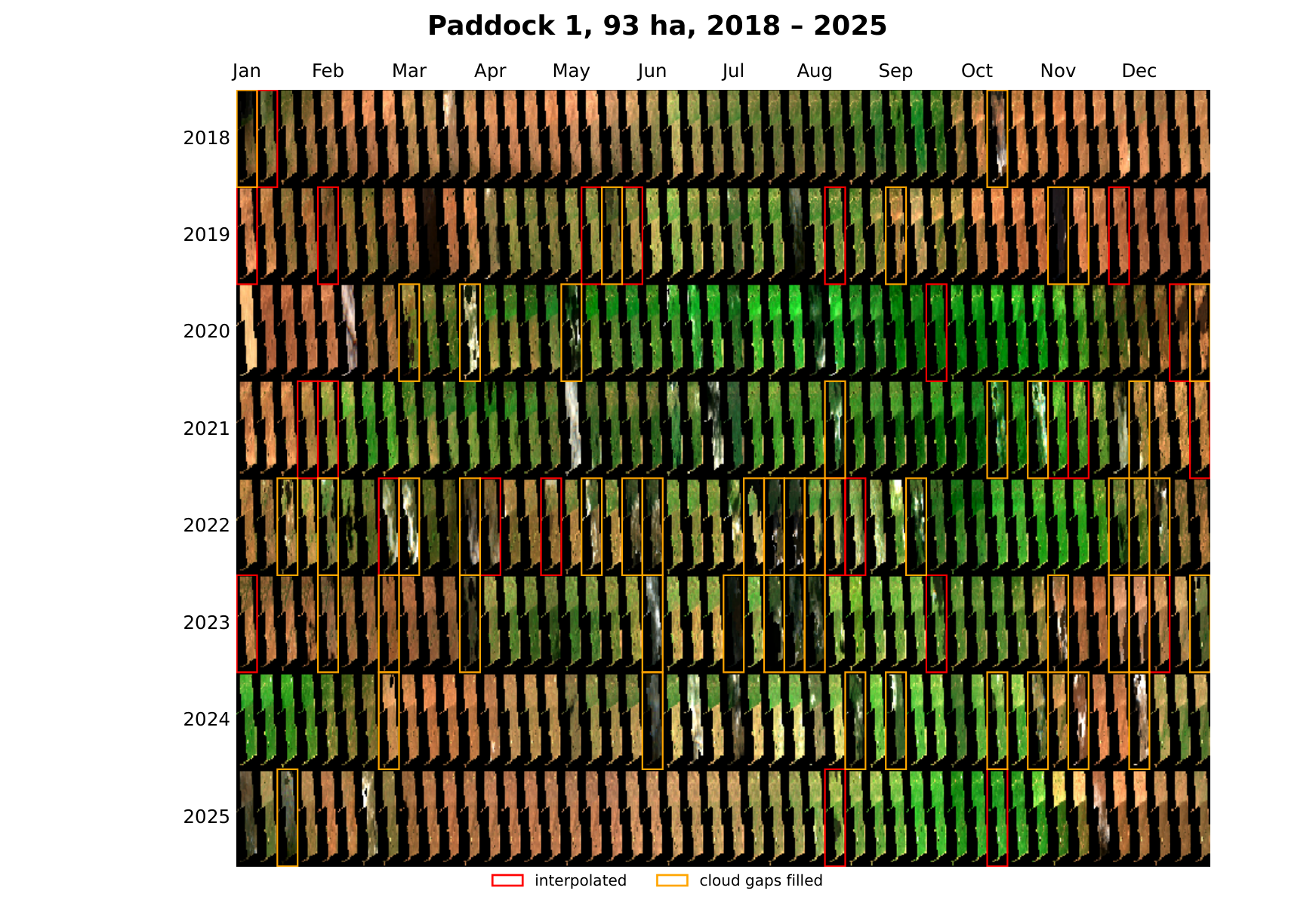 One page per paddock: each cell is the paddock's true-colour thumbnail
at that point in the season. Red outlines mark fully interpolated slots;
orange outlines mark observations whose cloud-masked pixels were gap-filled.
One page per paddock: each cell is the paddock's true-colour thumbnail
at that point in the season. Red outlines mark fully interpolated slots;
orange outlines mark observations whose cloud-masked pixels were gap-filled.
Stages 15–16: Phenology
estimate_phenology wraps the vendored
phenolopy library. For
each year and each paddock, it computes:
sos_times/sos_values— start of seasonpos_times/pos_values— peak of seasoneos_times/eos_values— end of season- amplitudes, length-of-season, integrals over season
num_peaks— independent count of identified seasons
Paddocks with fewer than min_observations (default 25) valid points
in a year are skipped for that year. The result is one tidy
pandas.DataFrame per year, returned as {year: DataFrame}.
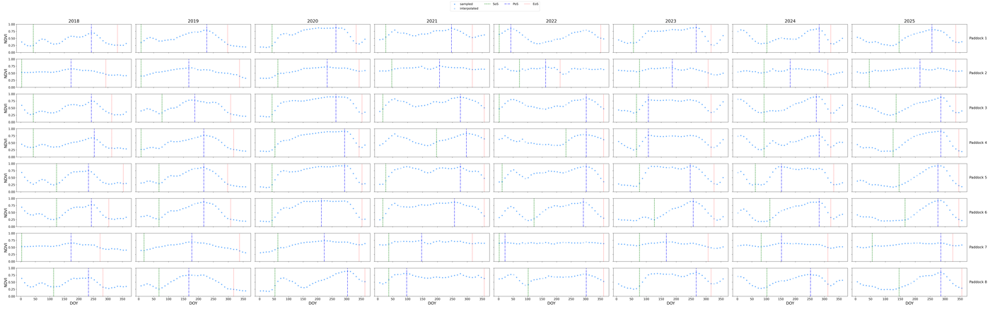 Smoothed NDVI with detected start / peak / end of season, per paddock per year.
Environmental data pipeline
Environmental data comes from the machine-wide store packages — each caches downloads across every troi on the machine, so overlapping regions and repeat runs re-fetch nothing:
| # | Stage | Store / module | Output |
|---|---|---|---|
| 1 | Download terrain (Copernicus DEM) | pycopdem |
elevation window (machine-wide store) |
| 2 | Download OzWALD daily | pyozwald |
daily meteorology (machine-wide store) |
| 3 | Download SILO climate | pysilo |
daily climate (machine-wide store) |
| 4 | Download SLGA soils | pyslga |
soil properties (machine-wide store) |
| 5 | DAESim forcing | PaddockTS.daesim_forcing |
{stub}_DAESim_forcing.csv |
| 6 | OzWALD plot | Plotting.ozwald_plot |
{stub}_ozwald_daily_*.png |
| 7 | SILO plot | Plotting.silo_plot |
{stub}_silo_*.png |
| 8 | Terrain plot | Plotting.terrain_tiles_plot |
{stub}_topography.png |
The terrain plot reprojects onto the Sentinel-2 pixel grid, which it reconstructs deterministically from the troi bbox — it does not wait on (or read) the Sentinel-2 data itself.
The SILO stages are silently skipped (status: skipped, not
error) if config.email is unset; the SLGA stage is skipped the
same way if config.tern_api_key is unset. Terrain and OzWALD work
without any credentials.
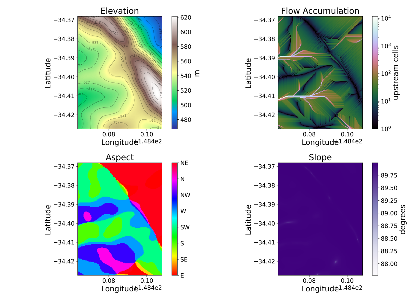 Elevation, flow accumulation, aspect, and slope derived from the
Copernicus DEM, reprojected onto the Sentinel-2 grid.
Elevation, flow accumulation, aspect, and slope derived from the
Copernicus DEM, reprojected onto the Sentinel-2 grid.
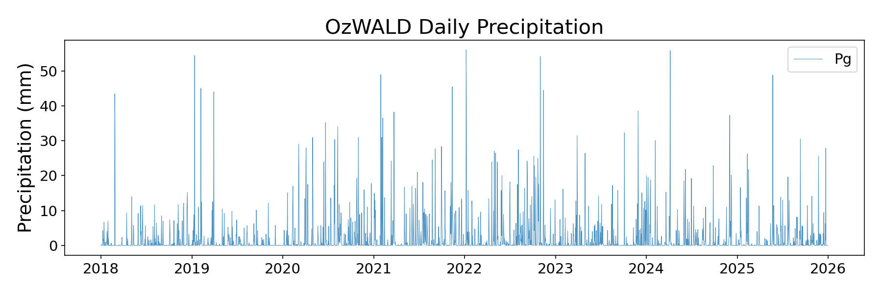 OzWALD daily climate diagnostic (one of several panels).
Skipping the dashboard
If you want one stage and don't need the live UI, call it directly —
nothing requires get_outputs:
The function loads (and if necessary downloads) its own inputs from the cache.
See also
- API reference — full function signatures with runnable examples
PaddockTS.get_outputs— the orchestratordiagnostics.md— known failure modes (DEA STAC cold-start, GDAL HTTP auth)