Phenology

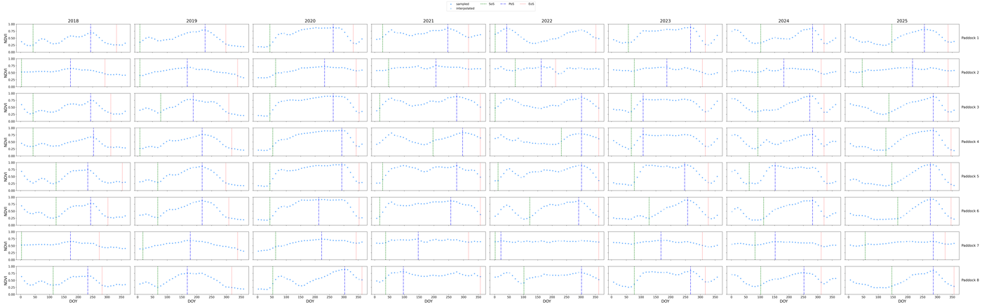
Per-paddock seasonal phenology metrics — start, peak, and end of season DOY plus amplitudes, length-of-season, and integrals — computed from a single vegetation-index time series.

SoS / PoS / EoS per paddock per year

The implementation wraps a vendored copy of phenolopy by Lewis Trotter (Apache 2.0-licensed; see PaddockTS/LICENSES/phenolopy.LICENSE). It lives at PaddockTS.Phenology._phenolopy with minor NumPy 2.0 compatibility fixes documented in the file header. A small monkey-patch is applied to xarray.merge during the call to silence a coordinate mismatch that upstream sees as a hard error.

---

Metrics returned

estimate_phenology returns {year: pandas.DataFrame}. Each DataFrame has one row per paddock and (among others) the following columns:

Column	Meaning
paddock	Paddock ID (string).
sos_times, sos_values	Start of season — DOY and vegetation-index value.
pos_times, pos_values	Peak of season — DOY and value.
eos_times, eos_values	End of season — DOY and value.
aos_values	Amplitude of season (peak − base).
los_values	Length of season in days.
sios_values	Small integral over season.
lios_values	Long integral over season.
num_peaks	Number of independent seasons / peaks detected.

See the phenolopy source for the full list. The exact column set depends on the peak_metric, base_metric, and method arguments (this module fixes them to pos / bse / seasonal_amplitude — edit the call to change).

---

Example: full call

from datetime import date
from troi.troi import Troi
from PaddockTS.Phenology.estimate_phenology import estimate_phenology

q = Troi(
    bbox=[148.36265, -33.52606, 148.38265, -33.50606],
    start=date(2022, 1, 1),
    end=date(2024, 12, 31),
    stub="phen_demo",
)

# Cascades: builds the yearly TS (and S2 / paddocks if needed)
results = estimate_phenology(q, variable="NDVI")

for year, df in results.items():
    print(f"\n{year} — {len(df)} paddocks")
    print(df[["paddock", "sos_times", "pos_times", "eos_times",
              "aos_values", "los_values", "num_peaks"]].head())

Sample output:

2023 — 12 paddocks
  paddock  sos_times  pos_times  eos_times  aos_values  los_values  num_peaks
0       1         85        178        262        0.61         177         1
1       2         92        184        268        0.55         176         1
2       3        102        205        290        0.48         188         1
...

---

Example: a different vegetation index

NIRv or CFI sometimes track productivity better than NDVI on low-LAI canopies or heterogeneous paddocks:

results_nirv = estimate_phenology(q, variable="NIRv")
results_cfi  = estimate_phenology(q, variable="CFI")

The selected variable must exist in the yearly time-series dataset (it does for any of NDVI, CFI, NIRv, NDTI, CAI because compute_indices writes all five by default).

---

Example: stricter observation threshold

By default paddocks with fewer than 25 valid observations in a year are skipped — for short date ranges or sparse acquisition windows you may want to relax this:

results = estimate_phenology(q, variable="NDVI", min_observations=10)

---

Example: pass in an already-built yearly TS

If you've already built the yearly time series (e.g. cached from a previous run), pass it in to skip the rebuild:

from PaddockTS.Phenology.make_yearly_paddock_time_series import make_yearly_paddock_time_series

yearly = make_yearly_paddock_time_series(q)        # cached if already built
results = estimate_phenology(q, ds_yearly=yearly)

---

Example: plot a phenology curve with SoS / PoS / EoS markers

import matplotlib.pyplot as plt

year = 2023
ds_y = yearly[year]
df = results[year]

paddock_id = "1"
row = df[df["paddock"].astype(str) == paddock_id].iloc[0]

fig, ax = plt.subplots(figsize=(10, 4))
ax.scatter(ds_y.doy, ds_y.NDVI.sel(paddock=paddock_id), color="blue", s=12)
ax.axvline(row.sos_times, color="green",  linestyle="--", label="SoS")
ax.axvline(row.pos_times, color="blue",   linestyle="-.", label="PoS")
ax.axvline(row.eos_times, color="red",    linestyle=":",  label="EoS")
ax.set_xlabel("DOY")
ax.set_ylabel("NDVI")
ax.set_title(f"Paddock {paddock_id} — {year}")
ax.legend()

For a multi-paddock × multi-year version of the same plot, see phenology_plot.

---

Reference

PaddockTS.Phenology.estimate_phenology.estimate_phenology

estimate_phenology(troi, ds_yearly=None, variable='NDVI', min_observations=25, paddocks_filepath=None)

Compute per-paddock phenology metrics for each year.

For each year in ds_yearly, this:

1. Selects variable (e.g. 'NDVI') and renames it to veg_index (phenolopy's expected variable name).
2. Calls :func:phenolopy.calc_num_seasons to count peaks.
3. Calls :func:phenolopy.calc_phenometrics with a seasonal-amplitude method (5% threshold, two-sided) to derive SoS / PoS / EoS and associated values.
4. Flattens the result into a tidy :class:pandas.DataFrame and attaches the peak count.

Parameters:

Name	Type	Description	Default
troi		The :class:troi.Troi.	required
ds_yearly		Optional {year: xarray.Dataset} mapping (typically from :func:PaddockTS.Phenology.make_yearly_paddock_time_series). If None, built on demand. Each dataset must have a doy coordinate.	None
variable		Name of the data variable to feed into phenolopy. Defaults to 'NDVI'; 'NIRv' and 'CFI' also work and are sometimes preferred for low-LAI canopies.	'NDVI'
min_observations		Minimum number of valid observations required per paddock. Paddocks with fewer are skipped. Default 25.	25

Returns:

Type	Description
	dict[int, pandas.DataFrame]: One DataFrame per year. Columns
	include the phenolopy metrics (sos_times, sos_values,
	pos_times, eos_times, etc.) plus num_peaks and a
	paddock identifier.